Sales Data Analysis

#data #dataanalysis #python #ETL
By Sergio Castro
About our dataset
We first import some packages that will help us throgh our analysis.
					import pandas as pd
import numpy as np
import matplotlib.pyplot as plt
import seaborn as sns

# In order to work with feather files , we install pyarrow package

!pip install pyarrow

Defaulting to user installation because normal site-packages is not writeable
Requirement already satisfied: pyarrow in c:\programdata\anaconda3\lib\site-packages (14.0.2)
Requirement already satisfied: numpy>=1.16.6 in c:\programdata\anaconda3\lib\site-packages (from pyarrow) (1.26.4)
					all_data = pd.read_feather(r"C:\Users\Sergio C\Desktop\Analisis\Sales-analysis/Sales_data.ftr")

all_data.head(6)

	Order ID	Product 	           Quantity Ordered	Price Each   	Order Date	        Purchase Address
0	176558	USB-C Charging Cable	            2	       11.95	04/19/19 08:46	917 1st St, Dallas, TX 75001
1	None           	None                   	None        	None	      None	                      None
2	176559	Bose SoundSport Headphones	        1	       99.99	04/07/19 22:30	682 Chestnut St, Boston, MA 02215
3	176560	Google Phone                    	1	        600	    04/12/19 14:38	669 Spruce St, Los Angeles, CA 90001
4	176560	Wired Headphones                 	1	       11.99	04/12/19 14:38	669 Spruce St, Los Angeles, CA 90001
5	176561	Wired Headphones                 	1	       11.99	04/30/19 09:27	333 8th St, Los Angeles, CA 90001

## The data contains hundreds of thousands of electronics store purchases broken down by month, product type, cost , purchase address, etc
Data cleaning and formatting
					all_data.isnull().sum() # checking out total missing values we have
Order ID            545
Product             545
Quantity Ordered    545
Price Each          545
Order Date          545
Purchase Address    545
dtype: int64

# since there 545 observations where entire row have missing value , we can drop these 545 rows

all_data = all_data.dropna(how="all")
					all_data.isnull().sum()

Order ID            0
Product             0
Quantity Ordered    0
Price Each          0
Order Date          0
Purchase Address    0
dtype: int64

# Let's check whether we have duplicate rows or not

all_data.duplicated()

0         False
2         False
3         False
4         False
5         False
          ...
186845    False
186846    False
186847    False
186848    False
186849    False
Length: 186305, dtype: bool
					all_data[all_data.duplicated()] # total 618 duplicate rows
	Order ID	Product	Quantity Ordered	Price Each	Order Date	Purchase Address
31	176585	Bose SoundSport Headphones	1	99.99	04/07/19 11:31	823 Highland St, Boston, MA 02215
1149	Order ID	Product	Quantity Ordered	Price Each	Order Date	Purchase Address
1155	Order ID	Product	Quantity Ordered	Price Each	Order Date	Purchase Address
1302	177795	Apple Airpods Headphones	1	150	04/27/19 19:45	740 14th St, Seattle, WA 98101
1684	178158	USB-C Charging Cable	1	11.95	04/28/19 21:13	197 Center St, San Francisco, CA 94016
...	...	...	...	...	...	...
186563	Order ID	Product	Quantity Ordered	Price Each	Order Date	Purchase Address
186632	Order ID	Product	Quantity Ordered	Price Each	Order Date	Purchase Address
186738	Order ID	Product	Quantity Ordered	Price Each	Order Date	Purchase Address
186782	259296	Apple Airpods Headphones	1	150	09/28/19 16:48	894 6th St, Dallas, TX 75001
186785	259297	Lightning Charging Cable	1	14.95	09/15/19 18:54	138 Main St, Boston, MA 02215
618 rows × 6 columns
					all_data = all_data.drop_duplicates() # Dropping all the duplicate rows
all_data.shape
(185687, 6)


all_data[all_data.duplicated()]
	Order ID	Product	Quantity Ordered	Price Each	Order Date	Purchase Address
Which is the best month for sale ?
Lets first understand what this term ‘best’ is all about : if any month has maximum sales, we will consider that as best
					all_data.head(2)

	Order ID      	Product	       Quantity Ordered 	Price Each	 Order Date 	Purchase Address
0	176558	USB-C Charging Cable	       2            	11.95	04/19/19 08:46	917 1st St, Dallas, TX 75001
2	176559	Bose SoundSport Headphones	   1	            99.99	04/07/19 22:30	682 Chestnut St, Boston, MA 02215

# add month column

all_data['Order Date'][0]
'04/19/19 08:46'

'04/19/19 08:46'.split(' ')[0]
'04/19/19'

'04/19/19 08:46'.split(' ')[0].split('/')[0] ## extracting month from "Order Date"
'04'

all_data['Order Date'][0].split('/')[0] ## extracting month from "Order Date"
'04'
					def return_month(x):
    return x.split('/')[0]

all_data['Month'] = all_data['Order Date'].apply(return_month) ## applying return_month function on top of "Order Date" feature

all_data.dtypes

Order ID            object
Product             object
Quantity Ordered    object
Price Each          object
Order Date          object
Purchase Address    object
Month               object
dtype: object

all_data['Month'].astype(int) ## convert dat-type into integer
					all_data['Month'].unique() ## checking unique months
array(['04', '05', 'Order Date', '08', '09', '12', '01', '02', '03', '07',
       '06', '11', '10'], dtype=object)

filter1 = all_data['Month'] == 'Order Date'
all_data[~filter1]

	Order ID	Product	Quantity Ordered	Price Each	Order Date	Purchase Address	Month
0	176558	USB-C Charging Cable	2	11.95	04/19/19 08:46	917 1st St, Dallas, TX 75001	04
2	176559	Bose SoundSport Headphones	1	99.99	04/07/19 22:30	682 Chestnut St, Boston, MA 02215	04
3	176560	Google Phone	1	600	04/12/19 14:38	669 Spruce St, Los Angeles, CA 90001	04
4	176560	Wired Headphones	1	11.99	04/12/19 14:38	669 Spruce St, Los Angeles, CA 90001	04
5	176561	Wired Headphones	1	11.99	04/30/19 09:27	333 8th St, Los Angeles, CA 90001	04
...	...	...	...	...	...	...	...
186845	259353	AAA Batteries (4-pack)	3	2.99	09/17/19 20:56	840 Highland St, Los Angeles, CA 90001	09
186846	259354	iPhone	1	700	09/01/19 16:00	216 Dogwood St, San Francisco, CA 94016	09
186847	259355	iPhone	1	700	09/23/19 07:39	220 12th St, San Francisco, CA 94016	09
186848	259356	34in Ultrawide Monitor	1	379.99	09/19/19 17:30	511 Forest St, San Francisco, CA 94016	09
186849	259357	USB-C Charging Cable	1	11.95	09/30/19 00:18	250 Meadow St, San Francisco, CA 94016	09
185686 rows × 7 columns
					all_data = all_data[~filter1] ## excluding all those rows which have entry as "Order Date" in month feature
all_data.shape
(185686, 7)
## use warnings package to get rid of any warnings ..

import warnings
from warnings import filterwarnings
filterwarnings('ignore')
					all_data['Month'] = all_data['Month'].astype(int)

all_data.dtypes
Order ID            object
Product             object
Quantity Ordered    object
Price Each          object
Order Date          object
Purchase Address    object
Month                int32
dtype: object
					all_data['Quantity Ordered'] = all_data['Quantity Ordered'].astype(int)
all_data['Price Each'] = all_data['Price Each'].astype(float)
all_data.dtypes
Order ID             object
Product              object
Quantity Ordered      int32
Price Each          float64
Order Date           object
Purchase Address     object
Month                 int32
dtype: object
					all_data['sales'] = all_data['Quantity Ordered'] * all_data['Price Each'] ## creating sales feature
all_data['sales']
0          23.90
2          99.99
3         600.00
4          11.99
5          11.99
           ...
186845      8.97
186846    700.00
186847    700.00
186848    379.99
186849     11.95
Name: sales, Length: 185686, dtype: float64
					all_data.groupby(['Month'])['sales'].sum()

Month
1     1821413.16
2     2200078.08
3     2804973.35
4     3389217.98
5     3150616.23
6     2576280.15
7     2646461.32
8     2241083.37
9     2094465.69
10    3734777.86
11    3197875.05
12    4608295.70
Name: sales, dtype: float64
all_data.groupby(['Month'])['sales'].sum().plot(kind='bar')
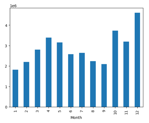
Viz. 1 Monthly sale comparison.
-y-axis scale : 1e^6
-E stands for exponential , in short it is *10^. So, 1e6 or 1e^6 OR 1 exponent 6 is the same as 1*10^6 which is same as 1,000,000
Inference : December is the best month of sales
Which city has max orders?
					all_data.head(2)
	Order ID	Product           	Quantity Ordered	Price Each	Order Date	Purchase Address    	          Month	sales
0	176558	USB-C Charging Cable	        2	          11.95	04/19/19 08:46	917 1st St, Dallas, TX 75001	    4	23.90
2	176559	Bose SoundSport Headphones	    1	          99.99	04/07/19 22:30	682 Chestnut St, Boston, MA 02215	4	99.99
					all_data['Purchase Address'][0]
'917 1st St, Dallas, TX 75001'

all_data['Purchase Address'][0].split(',')[1] ## extracting city from "Purchase Address"
' Dallas'

all_data['city'] = all_data['Purchase Address'].str.split(',').str.get(1)
all_data['city']
0                 Dallas
2                 Boston
3            Los Angeles
4            Los Angeles
5            Los Angeles
               ...
186845       Los Angeles
186846     San Francisco
186847     San Francisco
186848     San Francisco
186849     San Francisco
Name: city, Length: 185686, dtype: object
					pd.value_counts(all_data['city']) ## frequency table
city
San Francisco    44662
Los Angeles      29564
New York City    24847
Boston           19901
Atlanta          14863
Dallas           14797
Seattle          14713
Portland         12449
Austin            9890
Name: count, dtype: int64
pd.value_counts(all_data['city']).plot(kind='pie' , autopct = '%1.0f%%') ## Pandas pie chart..
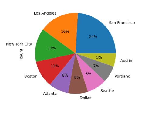
Viz. 2 Cities and their order %
-Inference : New York , Los Angeles , San Francisco are the Top 3 cities which has max order (53% all together)
What product sold the most?
					all_data.columns
Index(['Order ID', 'Product', 'Quantity Ordered', 'Price Each', 'Order Date',
       'Purchase Address', 'Month', 'sales', 'city'],
      dtype='object')
count_df = all_data.groupby(['Product']).agg({'Quantity Ordered':'sum' , 'Price Each':'mean'})
count_df = count_df.reset_index()

count_df

Product                         	Quantity Ordered	Price Each
0	20in Monitor                             	4126	109.99
1	27in 4K Gaming Monitor                  	6239	389.99
2	27in FHD Monitor                        	7541	149.99
3	34in Ultrawide Monitor                   	6192	379.99
4	AA Batteries (4-pack)	                   27615	3.84
5	AAA Batteries (4-pack)                     30986	2.99
6	Apple Airpods Headphones	               15637	150.00
7	Bose SoundSport Headphones	               13430	99.99
8	Flatscreen TV	                            4813	300.00
9	Google Phone	                            5529	600.00
10	LG Dryer	                                 646	600.00
11	LG Washing Machine                         	 666	600.00
12	Lightning Charging Cable	               23169	14.95
13	Macbook Pro Laptop	                        4725	1700.00
14	ThinkPad Laptop	                            4128	999.99
15	USB-C Charging Cable	                   23931	11.95
16	Vareebadd Phone	                            2068	400.00
17	Wired Headphones                           20524	11.99
18	iPhone	                                    6847	700.00
pd.value_counts(all_data['city']).plot(kind='pie' , autopct = '%1.0f%%') ## Pandas pie chart..
Note: In the context of Matplotlib, “twin axes” refers to the ability to create a figure with dual x-axes or y-axes, depending on the requirement.
plt.twinx(): This function creates a secondary y-axis that shares the same x-axis as the original plot. This is useful for comparing data with different scales on the same x-axis.
plt.twiny(): This function creates a secondary x-axis that shares the same y-axis as the original plot. It allows you to represent different scales or units along the x-axis while keeping the y-axis constant.
Understanding Trend of the most sold product ?
					all_data['Product'].value_counts()[0:5].index   ## Top 5 most sold products ..
Index(['USB-C Charging Cable', 'Lightning Charging Cable',
       'AAA Batteries (4-pack)', 'AA Batteries (4-pack)', 'Wired Headphones'],
      dtype='object', name='Product')

most_sold_product = all_data['Product'].value_counts()[0:5].index

all_data['Product'].isin(most_sold_product)

0          True
2         False
3         False
4          True
5          True
          ...
186845     True
186846    False
186847    False
186848    False
186849     True
Name: Product, Length: 185686, dtype: bool
					most_sold_product_df = all_data[all_data['Product'].isin(most_sold_product)]  ## data of Top 5 most sold products only
most_sold_product_df.head(4)

    Order ID	Product         	Quantity Ordered	Price Each	Order Date	      Purchase Address	                Month	sales	city
0	176558	USB-C Charging Cable	      2	               11.95	04/19/19 08:46	917 1st St, Dallas, TX 75001        	4	23.90	Dallas
4	176560	Wired Headphones	          1	               11.99	04/12/19 14:38	669 Spruce St, Los Angeles, CA 90001	4	11.99	Los Angeles
5	176561	Wired Headphones              1	               11.99	04/30/19 09:27	333 8th St, Los Angeles, CA 90001	    4	11.99	Los Angeles
6	176562	USB-C Charging Cable	      1	               11.95	04/29/19 13:03	381 Wilson St, San Francisco, CA 94016	4	11.95	San Francisco
					most_sold_product_df.groupby(['Month' , 'Product']).size()
Month  Product
1      AA Batteries (4-pack)       1037
       AAA Batteries (4-pack)      1084
       Lightning Charging Cable    1069
       USB-C Charging Cable        1171
       Wired Headphones            1004
2      AA Batteries (4-pack)       1274
       AAA Batteries (4-pack)      1320
       Lightning Charging Cable    1393
       USB-C Charging Cable        1511
       Wired Headphones            1179
3      AA Batteries (4-pack)       1672
       AAA Batteries (4-pack)      1645
       Lightning Charging Cable    1749
       USB-C Charging Cable        1766
       Wired Headphones            1512
4      AA Batteries (4-pack)       2062
       AAA Batteries (4-pack)      1988
       Lightning Charging Cable    2197
       USB-C Charging Cable        2074
       Wired Headphones            1888
5      AA Batteries (4-pack)       1821
       AAA Batteries (4-pack)      1888
       Lightning Charging Cable    1929
       USB-C Charging Cable        1879
       Wired Headphones            1729
6      AA Batteries (4-pack)       1540
       AAA Batteries (4-pack)      1451
       Lightning Charging Cable    1560
       USB-C Charging Cable        1531
       Wired Headphones            1334
7      AA Batteries (4-pack)       1555
       AAA Batteries (4-pack)      1554
       Lightning Charging Cable    1690
       USB-C Charging Cable        1667
       Wired Headphones            1434
8      AA Batteries (4-pack)       1357
       AAA Batteries (4-pack)      1340
       Lightning Charging Cable    1354
       USB-C Charging Cable        1339
       Wired Headphones            1191
9      AA Batteries (4-pack)       1314
       AAA Batteries (4-pack)      1281
       Lightning Charging Cable    1324
       USB-C Charging Cable        1451
       Wired Headphones            1173
10     AA Batteries (4-pack)       2240
       AAA Batteries (4-pack)      2234
       Lightning Charging Cable    2414
       USB-C Charging Cable        2437
       Wired Headphones            2091
11     AA Batteries (4-pack)       1970
       AAA Batteries (4-pack)      1999
       Lightning Charging Cable    2044
       USB-C Charging Cable        2054
       Wired Headphones            1777
12     AA Batteries (4-pack)       2716
       AAA Batteries (4-pack)      2828
       Lightning Charging Cable    2887
       USB-C Charging Cable        2979
       Wired Headphones            2537
dtype: int64
					pivot = most_sold_product_df.groupby(['Month' , 'Product']).size().unstack()

pivot.plot(figsize=(8,6))
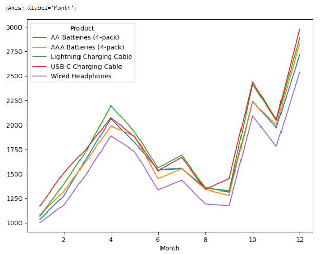
Viz. 3 Most sold product
-Inference : Products have been sold more in Oct , Nov , Dec with some good weeks between March-May.
What products are most often sold together ?
If we check orders that have same order Id, we can tell if they are sold mostly together.
Approach : i.e keep duplicated data
					all_data.columns
Index(['Order ID', 'Product', 'Quantity Ordered', 'Price Each', 'Order Date',
       'Purchase Address', 'Month', 'sales', 'city'],
      dtype='object')

all_data['Order ID']
0         176558
2         176559
3         176560
4         176560
5         176561
           ...
186845    259353
186846    259354
186847    259355
186848    259356
186849    259357
Name: Order ID, Length: 185686, dtype: object
					df_duplicated = all_data[all_data['Order ID'].duplicated(keep=False)]
df_duplicated # dataframe in which we have those Order Ids who have purchased more products

dup_products = df_duplicated.groupby(['Order ID'])['Product'].apply(lambda x : ','.join(x)).reset_index().rename(columns={'Product':'grouped_products'})

## for every Order-Id , collect all the products ..
					dup_products

	Order ID	grouped_products
0	141275	USB-C Charging Cable,Wired Headphones
1	141290	Apple Airpods Headphones,AA Batteries (4-pack)
2	141365	Vareebadd Phone,Wired Headphones
3	141384	Google Phone,USB-C Charging Cable
4	141450	Google Phone,Bose SoundSport Headphones
...	...	...
6874	319536	Macbook Pro Laptop,Wired Headphones
6875	319556	Google Phone,Wired Headphones
6876	319584	iPhone,Wired Headphones
6877	319596	iPhone,Lightning Charging Cable
6878	319631	34in Ultrawide Monitor,Lightning Charging Cable
6879 rows × 2 columns
					dup_products_df = df_duplicated.merge(dup_products , how='left' , on='Order ID') ## merge dataframes
no_dup_df = dup_products_df.drop_duplicates(subset=['Order ID']) # lets drop out all duplicate Order ID
no_dup_df.shape
(6879, 10)
no_dup_df['grouped_products'].value_counts()[0:5].plot.pie()
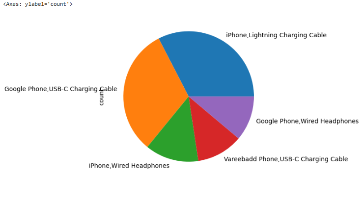
Viz. 4 Popular products bough together
-Inference :
When a person purchases an iPhone, we can immediately recommend complementary products, such as a charging cable or wired headphones. Similarly, when someone buys a Google phone, we can suggest a USB-C charging cable.
This is a critical insight for anyone designing a recommendation system, as it highlights the value of associating relevant accessories or add-ons with a primary purchase to enhance the customer experience and increase sales.
Conclusions
Analysis Summary:
From our analysis, we uncovered the following key insights:
- Top Ordering Cities: Identified the cities with the highest order volumes.
- Sales Trends by Month: Determined the best and worst months for sales.
- Product Popularity: Highlighted the most popular products and the optimal months to sell them.
- Popular Combos: Analyzed products frequently bought together to identify top-selling combinations.
Actionable Insights:
By leveraging these findings, we can:
- Develop targeted business strategies to boost sales in specific regions or time periods.
- Enhance our recommendation systems by suggesting complementary products, leading to increased revenue.
Thanks for your time.