S&P 500 Stock Market Analysis
#data #dataanalysis #python #ETL
By Sergio Castro
About our dataset
Through this analysis we will be exploring a dataset that containts the 5-Year stock record of 500 companies.
The Standard and Poor’s 500, or simply the S&P 500 is a stock market index tracking the stock performance of 500 of the largest companies listed on stock exchanges in the United States. It is one of the most commonly followed equity indices and includes approximately 80% of the total market capitalization of U.S. public companies, with an aggregate market cap of more than $43 trillion as of January 2024.
This analysis has two main objectives: to explore the available data and create useful visualizations, as well as to identify any correlations between the stock prices of different companies.
We first import some packages that will help us throgh our analysis.
					import pandas as pd
import numpy as np
import matplotlib.pyplot as plt
import seaborn as sns
import glob
We then connect our notebook to the local data we will be using to perform our stock analysis.
					glob.glob(r'C:\Users\Sergio C\Desktop\Analisis\Stock analysis\2-Time Series Data Analysis\individual_stocks_5yr/*csv')
# Here we are adding a *csv so we can pull all our cvs files on the local path.

len(glob.glob(r'C:\Users\Sergio C\Desktop\Analisis\Stock analysis\2-Time Series Data Analysis\individual_stocks_5yr/*csv'))
509 # Here we are just checking how many files we have.
After connecting our notebook to the data in question, we create a list that will only include those specific companies records we are interested in. We can now can iniate to explore our data and store specific information we need into perfom calculations.
					company_list = [
    r'C:\\Users\\Sergio C\\Desktop\\Analisis\\Stock analysis\\2-Time Series Data Analysis\\individual_stocks_5yr\\AAPL_data.csv' ,
    r'C:\\Users\\Sergio C\\Desktop\\Analisis\\Stock analysis\\2-Time Series Data Analysis\\individual_stocks_5yr\\AMZN_data.csv' ,
    r'C:\\Users\\Sergio C\\Desktop\\Analisis\\Stock analysis\\2-Time Series Data Analysis\\individual_stocks_5yr\\GOOG_data.csv' ,
    r'C:\\Users\\Sergio C\\Desktop\\Analisis\\Stock analysis\\2-Time Series Data Analysis\\individual_stocks_5yr\\MSFT_data.csv'
]

import warnings
from warnings import filterwarnings
filterwarnings('ignore') # This is just to ignore some warnings that may get our documents too long or harder to follow.
					all_data = pd.DataFrame() #here we are creating a dataframe leveraging our pandas package and our company list previusly created (company_list).

for file in company_list:

    current_df = pd.read_csv(file)

    all_data = pd.concat([current_df , all_data] , ignore_index=True)

    all_data.shape
    (4752, 7)
					all_data.head(6) # Some exploration to understand what kind of data we have available now.

         date	open	high       low	close	  volume	Name
0	2013-02-08	27.35	27.71	27.310	27.55	33318306	MSFT
1	2013-02-11	27.65	27.92	27.500	27.86	32247549	MSFT
2	2013-02-12	27.88	28.00	27.750	27.88	35990829	MSFT
3	2013-02-13	27.93	28.11	27.880	28.03	41715530	MSFT
4	2013-02-14	27.92	28.06	27.870	28.04	32663174	MSFT
5	2013-02-15	28.04	28.16	27.875	28.01	49650538	MSFT


all_data['Name'].unique() # We retrieve the unique values from the 'name' column to ensure it contains only the desired entries.
array(['MSFT', 'GOOG', 'AMZN', 'AAPL'], dtype=object)
Data Cleaning/Transformation
We ensure that our data is free of empty spaces and duplicate rows. Additionally, we double-check the data types to confirm accuracy and make necessary transformations when required.
					all_data.isnull().sum() # checking empty rows
date      0
open      0
high      0
low       0
close     0
volume    0
Name      0
dtype: int64

all_data.dtypes # checking data types
date       object
open      float64
high      float64
low       float64
close     float64
volume      int64
Name       object
dtype: object
					all_data['date'] = pd.to_datetime(all_data['date']) # Transforming our Date column from "object" to datetime64[ns]

all_data['date']
0      2013-02-08
1      2013-02-11
2      2013-02-12
3      2013-02-13
4      2013-02-14
          ...
4747   2018-02-01
4748   2018-02-02
4749   2018-02-05
4750   2018-02-06
4751   2018-02-07
Name: date, Length: 4752, dtype: datetime64[ns] #Here we can see the dtype changed
We then create a list (‘tech_list’) of the stocks we are interested in analyzing, each identified by its specific ticker symbol, such as MSFT for Microsoft, GOOG for Google, AMZN for Amazon, and AAPL for Apple.
					tech_list = all_data['Name'].unique()

tech_list
array(['MSFT', 'GOOG', 'AMZN', 'AAPL'], dtype=object)
With our data now organized and cleaned, we can leverage visualization libraries to create comparative visualizations of stock process over the years.
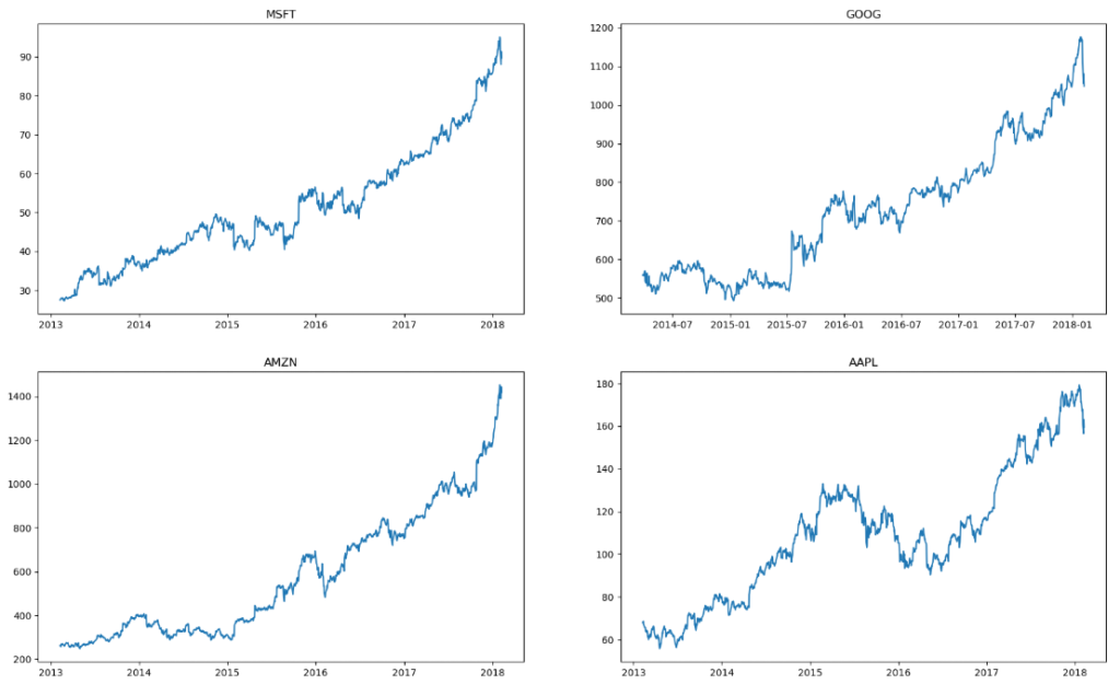
					plt.figure(figsize=(20,12)) # Here we are comparing different closing prices by leveraging our 'date' and 'close' columns.
for index , company in enumerate(tech_list , 1):
    plt.subplot(2 , 2 , index)
    filter1 = all_data['Name']==company
    df = all_data[filter1]
    plt.plot(df['date'] , df['close'])
    plt.title(company)
Viz 1. Stock closing price change over 5 years for each company.
- These visualizations enable us to easily identify the highest peaks in each stock’s record, providing valuable insights.
Now, an interesting question related to the stock market is: What were the moving averages of the various stocks?
					all_data.head(15) # Here we are just exploring our columns, here we can see that we have two columns named 'high' and 'low' and will help us with the question above.
          date	   open	 high	   low	 close	  volume	Name
0	2013-02-08	27.3500	27.71	27.310	27.550	33318306	MSFT
1	2013-02-11	27.6500	27.92	27.500	27.860	32247549	MSFT
2	2013-02-12	27.8800	28.00	27.750	27.880	35990829	MSFT
3	2013-02-13	27.9300	28.11	27.880	28.030	41715530	MSFT
4	2013-02-14	27.9200	28.06	27.870	28.040	32663174	MSFT
5	2013-02-15	28.0400	28.16	27.875	28.010	49650538	MSFT
6	2013-02-19	27.8801	28.09	27.800	28.045	38804616	MSFT
7	2013-02-20	28.1300	28.20	27.830	27.870	44109412	MSFT
8	2013-02-21	27.7400	27.74	27.230	27.490	49078338	MSFT
9	2013-02-22	27.6800	27.76	27.480	27.760	31425726	MSFT
10	2013-02-25	27.9700	28.05	27.370	27.370	48011248	MSFT
11	2013-02-26	27.3800	27.60	27.340	27.370	49917353	MSFT
12	2013-02-27	27.4200	28.00	27.330	27.810	36390889	MSFT
13	2013-02-28	27.8800	27.97	27.740	27.800	35836861	MSFT
14	2013-03-01	27.7200	27.98	27.520	27.950	34849287	MSFT


all_data['close'].rolling(window=10).mean().head(14) # When calculating the moving average, it is useful to ->
# -> compute it in segments. We can consider groups of 10, 20, or 30 results, defined by our 'window' parameter.
0         NaN
1         NaN
2         NaN
3         NaN
4         NaN
5         NaN
6         NaN
7         NaN
8         NaN
9     27.8535
10    27.8355
11    27.7865
12    27.7795
13    27.7565
Name: close, dtype: float64
					new_data = all_data.copy()
# We are now preparing our data so we can use Pandas to create a cool viz instead of using Matplot, just to have some fun.
ma_day = [10 ,20 , 50]

for ma in ma_day:
    new_data['close_'+str(ma)] = new_data['close'].rolling(ma).mean()

new_data.tail(7) #This is just a quick trick so we can avoid those NaN resuls we got above

              date	   open	    high	     low	close  	volume	    Name    close_10   close_20 	close_50
4745	2018-01-30	165.525	167.3700	164.7000	166.97	46048185	AAPL	174.263	174.3340	172.9460
4746	2018-01-31	166.870	168.4417	166.5000	167.43	32478930	AAPL	173.096	174.0925	172.8726
4747	2018-02-01	167.165	168.6200	166.7600	167.78	47230787	AAPL	171.948	173.8700	172.8252
4748	2018-02-02	166.000	166.8000	160.1000	160.50	86593825	AAPL	170.152	173.2435	172.6356
4749	2018-02-05	159.100	163.8800	156.0000	156.49	72738522	AAPL	168.101	172.3180	172.3026
4750	2018-02-06	154.830	163.7200	154.0000	163.03	68243838	AAPL	166.700	171.7520	172.0640
4751	2018-02-07	163.085	163.4000	159.0685	159.54	51608580	AAPL	165.232	171.0125	171.7554
new_data.set_index('date' , inplace=True)
					new_data
	         open	high	low	   close	volume	    Name	close_10	close_20	close_50
date
2013-02-08	27.350	27.71	27.3100	27.55	33318306	MSFT	NaN          	NaN          	NaN
2013-02-11	27.650	27.92	27.5000	27.86	32247549	MSFT	NaN         	NaN           	NaN
2013-02-12	27.880	28.00	27.7500	27.88	35990829	MSFT	NaN          	NaN	            NaN
2013-02-13	27.930	28.11	27.8800	28.03	41715530	MSFT	NaN	            NaN          	NaN
2013-02-14	27.920	28.06	27.8700	28.04	32663174	MSFT	NaN          	NaN          	NaN
...	...	...	...	...	...	...	...	...	...
2018-02-01	167.165	168.62	166.7600	167.78	47230787	AAPL	171.948	173.8700	172.8252
2018-02-02	166.000	166.80	160.1000	160.50	86593825	AAPL	170.152	173.2435	172.6356
2018-02-05	159.100	163.88	156.0000	156.49	72738522	AAPL	168.101	172.3180	172.3026
2018-02-06	154.830	163.72	154.0000	163.03	68243838	AAPL	166.700	171.7520	172.0640
2018-02-07	163.085	163.40	159.0685	159.54	51608580	AAPL	165.232	171.0125	171.7554
4752 rows × 9 columns
					new_data.columns
Index(['open', 'high', 'low', 'close', 'volume', 'Name', 'close_10',
       'close_20', 'close_50'],
      dtype='object')
					plt.figure(figsize=(24,18)) # This for cycle works similarly as the last one we used to create the last viz, we are just using Pandas instead of matplot

for index , company in enumerate(tech_list , 1):
    plt.subplot(2 , 2 , index)
    filter1 = new_data['Name']==company
    df = new_data[filter1]
    df[['close_10','close_20','close_50']].plot(ax=plt.gca())
    plt.title(company)
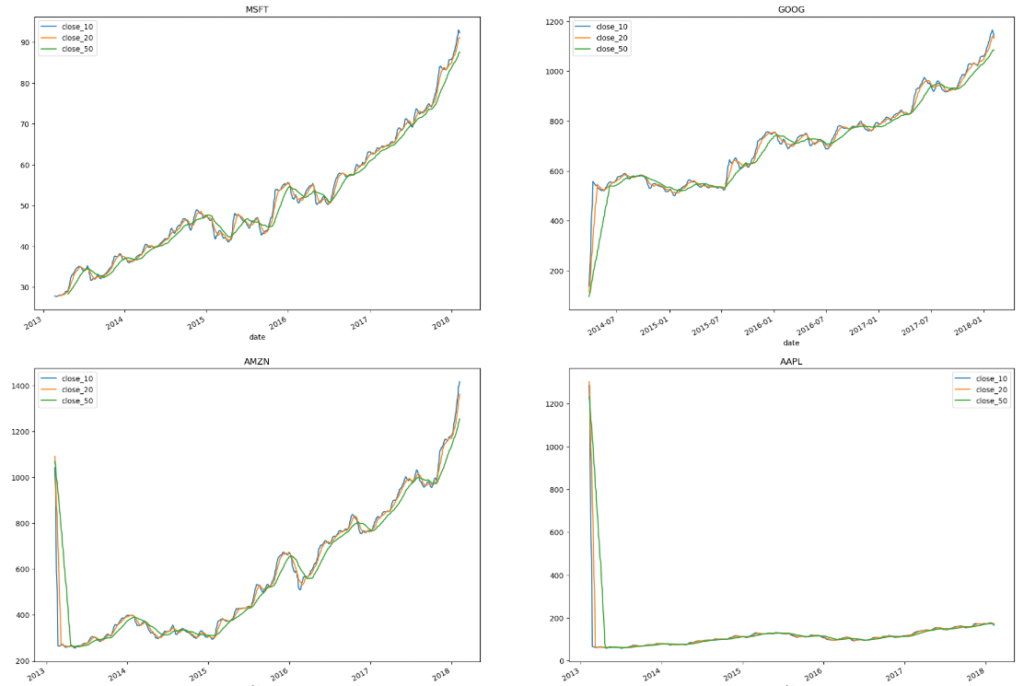
Viz 2. Stock moving average price change over 5 years for each company.
- These visualizations allow use to quickly compare different moving averages windows: 10, 20 and 50 days.
Let's analyze Apple closing prices change over time.
					apple = pd.read_csv( r'C:\\Users\\Sergio C\\Desktop\\Analisis\\Stock analysis\\2-Time Series Data Analysis\\individual_stocks_5yr\\AAPL_data.csv')

apple.head(4)

    	date	   open	   high	    low	  close 	volume	Name
0	2013-02-08	67.7142	68.4014	66.8928	67.8542	158168416	AAPL
1	2013-02-11	68.0714	69.2771	67.6071	68.5614	129029425	AAPL
2	2013-02-12	68.5014	68.9114	66.8205	66.8428	151829363	AAPL
3	2013-02-13	66.7442	67.6628	66.1742	66.7156	118721995	AAPL
					apple['close']

0        67.8542
1        68.5614
2        66.8428
3        66.7156
4        66.6556
          ...
1254    167.7800
1255    160.5000
1256    156.4900
1257    163.0300
1258    159.5400
Name: close, Length: 1259, dtype: float64
					apple['Daily return(in %)'] = apple['close'].pct_change()*100

apple.head(4)

          date	   open 	high	low	  close	  volume	Name	Daily return(in %)
0	2013-02-08	67.7142	68.4014	66.8928	67.8542	158168416	AAPL	NaN
1	2013-02-11	68.0714	69.2771	67.6071	68.5614	129029425	AAPL	1.042235
2	2013-02-12	68.5014	68.9114	66.8205	66.8428	151829363	AAPL	-2.506658
3	2013-02-13	66.7442	67.6628	66.1742	66.7156	118721995	AAPL	-0.190297
					import plotly.express as px

px.line(apple , x="date" , y="Daily return(in %)")
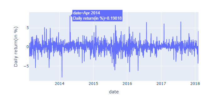
Viz 3. Apple stock change over time
- In this visualization, we observe several noticeable peaks over time. These peaks can be correlated with historical events, such as new product announcements.
Let's perform a resampling analysis.
What is resampling?
Resampling analysis is a statistical method that involves repeatedly sampling a dataset to estimate variability, test hypotheses, or aggregate data over specific intervals. Common techniques include bootstrapping, jackknifing, permutation testing, and time series resampling, often used in finance, forecasting, and model evaluation.
					apple.dtypes # First we will make sure that data is under the format we need.

date                   object
open                  float64
high                  float64
low                   float64
close                 float64
volume                  int64
Name                   object
Daily return(in %)    float64
dtype: object
					apple['date'] = pd.to_datetime(apple['date'])

apple.dtypes

date                  datetime64[ns] #Here can see the changes.
open                         float64
high                         float64
low                          float64
close                        float64
volume                         int64
Name                          object
Daily return(in %)           float64
dtype: object
					apple.head(4)

          date	   open	   high  	low	  close	   volume	Name	Daily return(in %)
0	2013-02-08	67.7142	68.4014	66.8928	67.8542	158168416	AAPL	NaN
1	2013-02-11	68.0714	69.2771	67.6071	68.5614	129029425	AAPL	1.042235
2	2013-02-12	68.5014	68.9114	66.8205	66.8428	151829363	AAPL	-2.506658
3	2013-02-13	66.7442	67.6628	66.1742	66.7156	118721995	AAPL	-0.190297

apple.set_index('date' , inplace=True) # here we are just setting a different index to work easier with our data.
					apple.head(4) #We can see that here we no longer have the first column and indexes have changed.

               open	   high  	low 	close	volume	Name	Daily return(in %)
date
2013-02-08	67.7142	68.4014	66.8928	67.8542	158168416	AAPL	NaN
2013-02-11	68.0714	69.2771	67.6071	68.5614	129029425	AAPL	1.042235
2013-02-12	68.5014	68.9114	66.8205	66.8428	151829363	AAPL	-2.506658
2013-02-13	66.7442	67.6628	66.1742	66.7156	118721995	AAPL	-0.190297
					apple['close'].resample('M').mean()
date
2013-02-28     65.306264
2013-03-31     63.120110
2013-04-30     59.966432
2013-05-31     63.778927
2013-06-30     60.791120
                 ...
2017-10-31    157.817273
2017-11-30    172.406190
2017-12-31    171.891500
2018-01-31    174.005238
2018-02-28    161.468000
Freq: ME, Name: close, Length: 61, dtype: float64
apple['close'].resample('M').mean().plot()
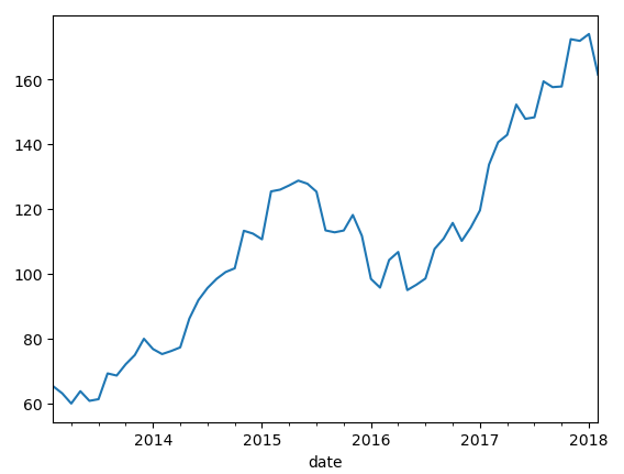
Viz 4. Apple change over time.
- In this visualization, we resampled our data on a monthly basis. The approach is flexible, allowing us to modify the code to generate similar results using different time windows, such as quarterly, weekly, or yearly intervals.
Are all these companies closing stock prices correlated?
Let’s perform a correlation analysis to identify relationships between stock price changes among the previously mentioned companies.
					company_list
['C:\\\\Users\\\\Sergio C\\\\Desktop\\\\Analisis\\\\Stock analysis\\\\2-Time Series Data Analysis\\\\individual_stocks_5yr\\\\AAPL_data.csv',
 'C:\\\\Users\\\\Sergio C\\\\Desktop\\\\Analisis\\\\Stock analysis\\\\2-Time Series Data Analysis\\\\individual_stocks_5yr\\\\AMZN_data.csv',
 'C:\\\\Users\\\\Sergio C\\\\Desktop\\\\Analisis\\\\Stock analysis\\\\2-Time Series Data Analysis\\\\individual_stocks_5yr\\\\GOOG_data.csv',
 'C:\\\\Users\\\\Sergio C\\\\Desktop\\\\Analisis\\\\Stock analysis\\\\2-Time Series Data Analysis\\\\individual_stocks_5yr\\\\MSFT_data.csv']
					company_list[0]
'C:\\\\Users\\\\Sergio C\\\\Desktop\\\\Analisis\\\\Stock analysis\\\\2-Time Series Data Analysis\\\\individual_stocks_5yr\\\\AAPL_data.csv'

app = pd.read_csv(company_list[0])
amzn = pd.read_csv(company_list[1])
google = pd.read_csv(company_list[2])
msft = pd.read_csv(company_list[3])

closing_price = pd.DataFrame()

closing_price['apple_close'] = app['close']
closing_price['amzn_close'] = amzn['close']
closing_price['google_close'] = google['close']
closing_price['msft_close'] = msft['close']
					closing_price

	apple_close	amzn_close	google_close	msft_close
0	67.8542	261.95	558.46	27.55
1	68.5614	257.21	559.99	27.86
2	66.8428	258.70	556.97	27.88
3	66.7156	269.47	567.16	28.03
4	66.6556	269.24	567.00	28.04
...	...	...	...	...
1254	167.7800	1390.00	NaN	94.26
1255	160.5000	1429.95	NaN	91.78
1256	156.4900	1390.00	NaN	88.00
1257	163.0300	1442.84	NaN	91.33
1258	159.5400	1416.78	NaN	89.61
1259 rows × 4 columns
sns.pairplot(closing_price)
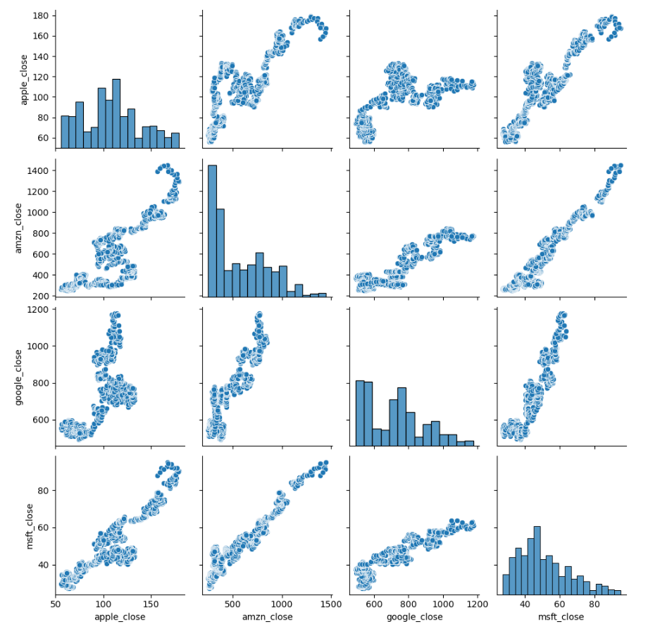
Viz 5. Correlation Pairplot.
- On this visualization we can easily notice that there’s a strong correlation between Microsoft/Amazon stock changes as they are the closer among x/y axis comparison.
But, how about a heatmap?
By adding some color to the mix, heatmaps make it easier to identify correlations among different concepts.
					closing_price.corr()

           	apple_close	amzn_close	google_close	msft_close
apple_close	1.000000	0.819078	0.640522	0.899689
amzn_close	0.819078	1.000000	0.888456	0.955977
google_close 0.640522	0.888456	1.000000	0.907011
msft_close	0.899689	0.955977	0.907011	1.000000
sns.heatmap(closing_price.corr() , annot=True)
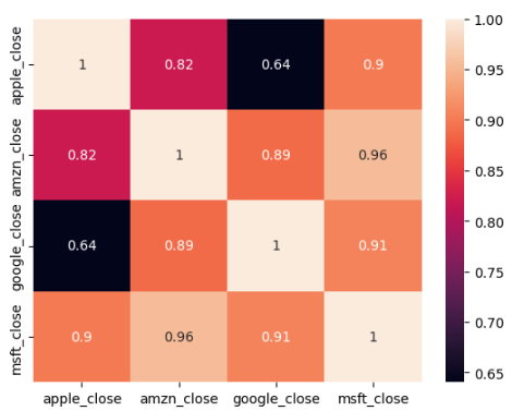
Viz 6. Correlation heatmap.
- On this visualization we can confirm that there’s a strong correlation between Microsoft/Amazon stock (0.96). Also, is easier to spot those that have no strong relation like the ones in black.
Let's end with a pairgrid.
					closing_price

	apple_close	amzn_close	google_close	msft_close
0	67.8542	261.95	558.46	27.55
1	68.5614	257.21	559.99	27.86
2	66.8428	258.70	556.97	27.88
3	66.7156	269.47	567.16	28.03
4	66.6556	269.24	567.00	28.04
...	...	...	...	...
1254	167.7800	1390.00	NaN	94.26
1255	160.5000	1429.95	NaN	91.78
1256	156.4900	1390.00	NaN	88.00
1257	163.0300	1442.84	NaN	91.33
1258	159.5400	1416.78	NaN	89.61
1259 rows × 4 columns
					closing_price['apple_close']

0        67.8542
1        68.5614
2        66.8428
3        66.7156
4        66.6556
          ...
1254    167.7800
1255    160.5000
1256    156.4900
1257    163.0300
1258    159.5400
Name: apple_close, Length: 1259, dtype: float64
					closing_price['apple_close'].shift(1)

0            NaN
1        67.8542
2        68.5614
3        66.8428
4        66.7156
          ...
1254    167.4300
1255    167.7800
1256    160.5000
1257    156.4900
1258    163.0300
Name: apple_close, Length: 1259, dtype: float64
					(closing_price['apple_close'] - closing_price['apple_close'].shift(1))/closing_price['apple_close'].shift(1)*100

0            NaN
1       1.042235
2      -2.506658
3      -0.190297
4      -0.089934
          ...
1254    0.209043
1255   -4.339015
1256   -2.498442
1257    4.179181
1258   -2.140710
Name: apple_close, Length: 1259, dtype: float64
					for col in closing_price.columns:
    closing_price[col + '_pc_change'] = (closing_price[col] - closing_price[col].shift(1))/closing_price[col].shift(1)*100

    closing_price

    	apple_close	amzn_close	google_close	msft_close	apple_close_pc_change	amzn_close_pc_change	google_close_pc_change	msft_close_pc_change
0	67.8542	261.95	558.46	27.55	NaN         NaN         	NaN	      NaN
1	68.5614	257.21	559.99	27.86	1.042235	-1.809506	0.273968	1.125227
2	66.8428	258.70	556.97	27.88	-2.506658	0.579293	-0.539295	0.071788
3	66.7156	269.47	567.16	28.03	-0.190297	4.163123	1.829542	0.538020
4	66.6556	269.24	567.00	28.04	-0.089934	-0.085353	-0.028211	0.035676
...	...	...	...	...	...	...	...	...
1254	167.7800	1390.00	NaN	94.26	0.209043	-4.196734	NaN	-0.789391
1255	160.5000	1429.95	NaN	91.78	-4.339015	2.874101	NaN	-2.631021
1256	156.4900	1390.00	NaN	88.00	-2.498442	-2.793804	NaN	-4.118544
1257	163.0300	1442.84	NaN	91.33	4.179181	3.801439	NaN	3.784091
1258	159.5400	1416.78	NaN	89.61	-2.140710	-1.806160	NaN	-1.883280
1259 rows × 8 columns
					closing_price.columns

Index(['apple_close', 'amzn_close', 'google_close', 'msft_close',
       'apple_close_pc_change', 'amzn_close_pc_change',
       'google_close_pc_change', 'msft_close_pc_change'],
      dtype='object')
					clsing_p = closing_price[['apple_close_pc_change', 'amzn_close_pc_change',
       'google_close_pc_change', 'msft_close_pc_change']]
					clsing_p

	apple_close_pc_change	amzn_close_pc_change	google_close_pc_change	msft_close_pc_change
0	NaN	NaN	NaN	NaN
1	1.042235	-1.809506	0.273968	1.125227
2	-2.506658	0.579293	-0.539295	0.071788
3	-0.190297	4.163123	1.829542	0.538020
4	-0.089934	-0.085353	-0.028211	0.035676
...	...	...	...	...
1254	0.209043	-4.196734	NaN	-0.789391
1255	-4.339015	2.874101	NaN	-2.631021
1256	-2.498442	-2.793804	NaN	-4.118544
1257	4.179181	3.801439	NaN	3.784091
1258	-2.140710	-1.806160	NaN	-1.883280
1259 rows × 4 columns
					g = sns.PairGrid(data= clsing_p)
g.map_diag(sns.histplot)
g.map_lower(sns.scatterplot)
g.map_upper(sns.kdeplot)
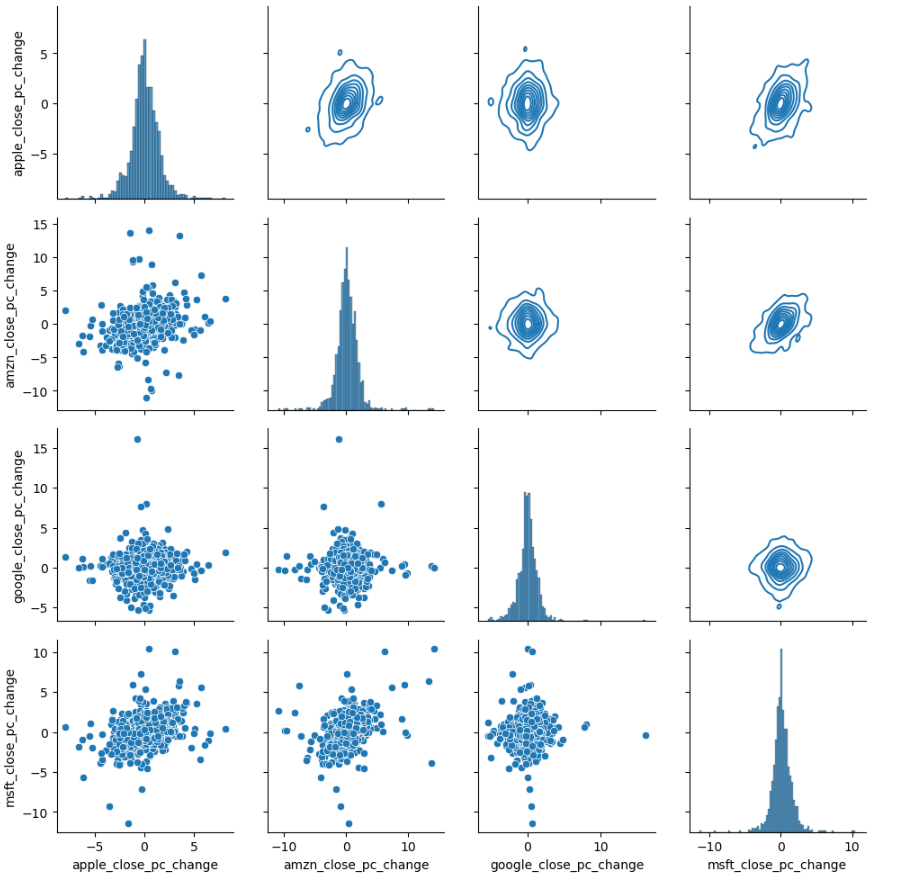
Viz 7. Pair Grid.
- This visualization allows us to compare different types of graphs, each providing unique insights into our data.
					clsing_p.corr()

                  	apple_close_pc_change	amzn_close_pc_change	google_close_pc_change	msft_close_pc_change
apple_close_pc_change	1.000000	             0.287659	                0.036202	           0.366598
amzn_close_pc_change	0.287659	             1.000000	                0.027698	           0.402678
google_close_pc_change	0.036202	             0.027698	                1.000000	           0.038939
msft_close_pc_change	0.366598                 0.402678	                0.038939            	1.000000
Conclusions.
By considering the last prompt after closing_p.corr(), we can observe different results. These results represent correlation scores between two companies’ stocks. For example, a score of 0.40 between MSFT and AMZN indicates a 40% likelihood that when one stock decreases, the other will also decrease. All the information and visuals obtained from this analysis provide highly valuable insights that can later be used to make informed decisions. Thank you for your time